Note:  This post is very long (1900 words) and involves some abstract strategic theory.  It is by no means a finished product, so I apologize if things aren’t very clear just yet.  Hopefully a few of you will read this and see where I’m going, in which case I’d love your help on explaining it better.  I have more to say about this, but I had to cut myself off somewhere.

Back in July, I wrote a post entitled “Not All Yards Are Created Equal“, which explained how team’s incentives and strategy should shift according to down and distance.  Today, I want to look at another area, with a thesis that will sound similar:

Not All Points Are Created Equal

Basically, points are not a static object; their “value” is not constant.  Of course, a TD is worth 6 points regardless of when you score it, but the VALUE of that TD changes.  The value of points, in essence, is a function of the relative strength of each team, the time remaining in the game, and the current conditions (Score/Field Position) of the game.

As those variables change, so to will the actual value of each point.  To make things easier, I’ve put those variables into an equation.  Note that this equation is not meant to be a “rule” or even be of any specific use.  It’s just to allow us to easily visualize what the relative consequences of variable changes will be to the overall result.

Expected Result = Relative Strength (1 – Time Elapsed / 60) + Current Position + Unknowns

OR

E = R ((60 – T) / 60) + C

Here, Expected Result is obviously the end result of the game.  Time Elapsed is similarly self-explanatory.  Current Position is a combination of the score and field position; here it may be helpful to think of AdvancedNFLStats.com’s Live Win Probability and each point during the game.  I’m going to ignore the Unknown factor because….well because its unknown.  We can’t quantify it; it’s just meant to serve as a reminder that a significant part of the outcome will be determined by chance.

Lastly, and most importantly (for my purposes today), is Relative Strength.  This factor accounts for the discrepancy in skill between the two teams.  Naturally, it’s difficult to quantify, which may be why NFL Coaches seems to be ignoring it in their in-game strategy, which brings me to my next major point:

NFL Coaches are ignoring a significant strategic factor in their in-game strategy, namely, Relative Strength.

Let’s look at Relative Strength at a high level, then drill a little deeper for practicality.  Using a timely example, this weeks Broncos vs. Jaguars game, we can easily see the importance of Relative Strength in in-game strategy.  For example, if the score at the end of the 1st quarter is Jax – 3, Denver – 0, who do you think will win?

Still Denver, right?  My guess is you’re also pretty confident about that.  So despite Jacksonville having a lead we still expect them to lose.  Why?  Because the Relative Strength is tilted so heavily in Denver’s favor that we expect them to outperform Jacksonville by a lot more than 3 points over the remaining 3 quarters.

Hopefully now you’re all with me.  Let’s go a little deeper, dipping our toes into Bayesian waters…

Relative Strength

The Relative Strength variable really consists of two components.  The first, and easiest to understand, is the ex-ante positioning of the teams.  For simplicity’s sake, we can use the Spread as a proxy.  There’s probably a better measure (Vegas isn’t trying to predict the outcomes), but, for you efficient market fans, it’s a pretty good representation of what we “know” about the relative strength of the participants before the game starts.

Going back to the Eagles/Broncos game, I believe the value was 11 points, in favor of Denver.  So, at that point, given all the information we knew about both the Broncos and Eagles, we (the market) expected that over 60 minutes of play, the Broncos would outperform the Eagles by 11 points.

Still with me?  Good, because now we get to the crux of the problem.

When the opening kick-off occurs, NFL Coaches seem to completely disregard that part of the R factor.  Instead, their conception of R is immediately replaced by the second component, New Information.  Essentially, NFL Coaches are overweighting the most recent data (what has happened in the game to that point) to the detriment of the other component of R, the ex-ante value.  This has very significant implications for in-game strategy, especially when the teams involved are of different skills levels.

To see why, let’s go back to our Jacksonville – Denver example.  The Spread for this week’s game, as of this writing, is 27 points (a record).  Using that as a proxy for R, we can write the original equation as follows, with a positive result (E) favoring Denver and a negative result favoring Jacksonville:

E = R ((60 – T) / 60) + C

E = 27 ((60-0) / 60) + 0

E = 27

Easy enough.  Now let’s look at our Jacksonville up 3 at the end of the 1Q scenario.

E = R ((60 – T) / 60) + C

E = 27 ((60-15) / 60) – 3

E = 27 ((45 / 60) – 3

E = 20.25 – 3

E = 17.25

Note that, for simplicity’s sake (again), I haven’t accounted for the second component of R, new information.  Doing so, in this situation, will lower R.  Our pre-game data pointed to an R of Denver +27, but we now have another quarter of play to account for.  Since Jacksonville won that quarter, the value of R has to drop.  HOWEVER, the point here is that, as a percentage of the overall sample, 1Q is pretty small, meaning the corresponding shift should be small as well, and definitely not large enough to account for the +17.25 value above.

So…Jacksonville is up 3-0 at the end of 1Q, but we still expect Denver to win by 17.25 points (a little less once we account for the New Information).  In your estimation, is that a “successful” quarter for Jacksonville?  Kind of.  They did significantly lower E (remember it has to go negative for JAX to win).  However, they’re still 17 points behind!

So, because R is so heavily tilted against them (Denver is much better), 3 points didn’t help that much…

Now we can start to see the foundation for my original assertion: Not all points are created equal.

Now let’s pretend that Jacksonville had a 4th and 3 at the 20 yard line when it kicked that FG (I haven’t run the EP scenario, pretend its equal, that is, kicking and going for it have the same expected value).  What should the team do?  GO FOR IT!

Over any amount of time, Denver is expected to significantly outplay Jacksonville.  That means that, up 3-0 at the end of 1Q, Jacksonville is still losing!  Let’s pretend for a minute that, after incorporating New Information, R is now equal to +16 (down from +17.25).  Should Jacksonville be confident, knowing they need to outplay Denver by 16 points over the rest of the game?  OF COURSE NOT!

When the Relative Strength of the participant teams is so uneven, the losing team must play AGGRESSIVELY, because at any time during the game, they should expect the other team to outplay them the rest of the way.  Therefore, to win, they need a large enough lead to account for the expected discrepancy.

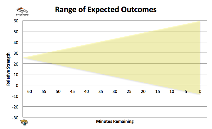
Let’s visualize it.

That’s an illustration of what we’d expect from two evenly matched teams.  We can argue over the size of the shaded area, but I didn’t put too much though into it, so let’s not dwell on it.

Now, let’s adjust it for the scenario we’ve been talking about.

Given that we’ve already incorporated relative strength (by setting the point at T= 60 to 27) and, theoretically, reflected all potential outcomes with our shaded area, we can project the progress of the game as a “random walk”, albeit one within the boundaries of the shaded area.

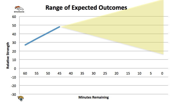
As the game progresses, the area will shift from left to right (time) and up/down (as R and C change).  Additionally, the width of the area will narrow, since less time remaining will progressively limit the range of outcomes.  So after the 1Q, it will look like this:

Notice that in this illustration, the odds of Jacksonville winning (shaded area below the x-axis) are still very small.  Given our ex-ante positioning, and what I believe is its proper inclusion in the in-game strategy, Jacksonville needs to do something significant if it hopes to have a reasonable chance of winning.  At this point, I need to step back and explain another aspect of the equation:

E = R ((60 – T) / 60) + C

Notice that as the game progresses, T converges to 0.  Logically, this makes complete sense.  With 30 seconds left in the game, the Relative Strength that we discussed above means almost nothing, there’s no time left for either team do much.  Conversely, C becomes more and more important, eventually becoming the only term (remember at the end of the game E = C).

So if we take our starting position, E = 27, and do nothing except run time off the clock, eventually that ex-ante advantage for Denver will disappear.  The point, though, is that we can’t forget it earlier in the game.

In current “conventional wisdom”, it’s almost as though once the game starts, R is forgotten; it shouldn’t be.

Over the course of the game, teams (especially bad ones) can only expect to have a couple of chances to significantly swing the odds (alter C).  To the degree that they are already behind (R), they should be more aggressive in effecting C, particularly because of one point:  You can, practically speaking, lose the game before the clock hits 0.  Using our illustration above, this would occur when the entire shaded area is above or below the x-axis.  So, let’s say the Broncos lead 21 – 0 at the end of the 1st Quarter.  It would look like this:

In the above illustration, using our equation, Jacksonville has already lost.  Basically, it will be nearly impossible for the Jaguars to outperform the Broncos by more than 21 points over the remaining 3 quarters, by virtue of what we know about their Relative Strength.

The takeaway is obvious.  The Jaguars can’t let it get to that point, hence kicking a FG instead of going for a TD in the red zone is a poor decision.  Again, we’ve accounted for relative strength in the positioning of the shaded area (range of outcomes), from there on in, the progression of the game should be thought of as random.  The Jaguars (and any significant underdog) need to take every opportunity they can to shift the range of outcomes.  They won’t get many chances, and in fact should never EXPECT to get another one.

So possession of the football in the red zone should be viewed as a singular and extremely valuable/important opportunity, once that should one that shouldn’t be wasted on a marginal gain of 3 points.

Going back to the beginning, the “value” of points changes according to the opponent.  3 Points against the Giants are worth far more than 3 points against the Broncos.  Coaches should adjust they’re strategy accordingly, and be much more aggressive when facing great teams.

The downside is that you don’t convert, and the range of outcomes shifts away from you. However, when there’s a significant mismatch, you were likely going to lose anyway.  By playing “conservatively”, i.e. taking the FG, you’re not only delaying the somewhat inevitable, but you’re passing on an important opportunity to make the game competitive.

Enough rambling…this needs a lot of refinement, but I had to start somewhere.  I know I still need to address assimilating New Information, so don’t think I’m ignoring it.  But I’ve lost 90% of the readers by now anyway, so I feel compelled to give the rest of you a temporary reprieve.